Как выбрать гостиницу для кошек
14 декабря, 2021
Сегодня каждый, кто собирается в отпуск и не знает, с кем оставить своего котика или кошку, может во[...]
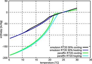
A series of measurements has been carried out with water as reference. Subsequently an emulsion produced by Fraunhofer Institute for Environmental-, Safety — and Energy Technologies (UMSICHT) was tested. This emulsion consists of 30% PCM (RT20) and 70% water. The melting enthalpy is about 60 kJ/kg over a temperature range of approximately 10 K (between 12 °C and 22 °C). Related to the melting temperature range this corresponds to a heat capacity of only 6 kJ/kgK which is only 1,43 times the value of water.
|
Fig. 2: The integrated heat flux curve for the pure RT20 and the utilized emulsion with 30% of the material during cooling and heating; measured with a Calvet-DSC |
|
|
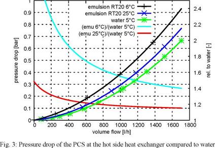
An important figure to evaluate the practicability of a PCS is its viscosity and the resulting pressure drops over different components. If the viscosity is much higher than the one of water, the advantage of higher energy density of PCS may be compensated by the higher hydraulic power necessary for pumping it. Also higher viscosities lead to reduced heat transfer in heat exchangers as the flow tends to laminar regime. Therefore the pressure drop of the phase change emulsion at the hot side heat exchanger was measured and compared to water as shown in Figure 3. The PCS was tested at two temperatures: at 5 °C as it is considered that all the PCM is in solid state and at 25 °C for molten PCM. As expected the viscosity is higher when the PCM is frozen, approximately by 20%. At low flow rates the relative pressure difference compared to water is high; at flow rates with practical relevance (above 300l/h) it takes values between 1,2 and 2. In a real application the PCM will melt or freeze within the heat exchanger, so the real pressure difference will lie between the obtained results.
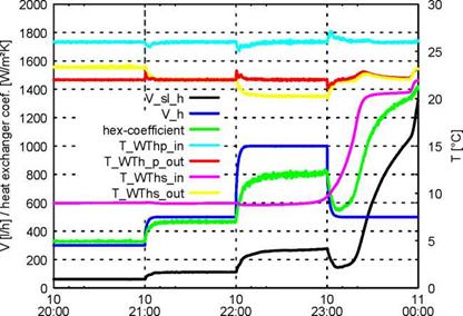
The following measurement was performed simulating a cooling application with 22 °C supply temperature and 26 °C return temperature, so the entire melting range of the material could be used. The storage was cooled down to 10 °C and the chiller then switched off. The heater was set to maintain the 26 °C. For the flow rate in the heating (load) circuit the following profile was defined: 300 l/h — 500 l/h — 1000 l/h — 500 l/h for an hour each, starting at 20:00 (equivalent to approx. 1390 W — 2320 W — 4640 W — 2320 W). The slurry pump was then controlled in such way that the 22 °C supply temperature was maintained independently of the flow rate in the heating circuit.
|
time [day of measurement H:M] Fig. 4: Measured values at the hot side heat exchanger: V_sl_h — slurry flow rate, V_h — heater flow rate, hex- coefficient — heat transfer coefficient, T_WThp_in/out — in-/ outlet temperature of the heater side of the heat exchanger, T_WThs_in/out — in-/ outlet temperature of the slurry side of the heat exchanger |
Figure 4 shows that during the first 3 hours the supply temperature (T_WThp_out) can be maintained constant with low slurry flow rates which means the heat can well be transferred to the slurry. A little before 23:00 the slurry temperature (T_WThs_in) starts to rise, so the controller increases the flow rate in the slurry circuit. The heat transfer coefficient is proportional to the volume flow rate, so the set temperature can be maintained although the temperature difference decreases. Shortly before 24:00 the
storage is entirely discharged, which the controller tries to compensate by setting the pump to full speed.
|
25 |
![]()
|
5 |
![]()
|
10 18:00 |
![]()
|
10 10 10 20:00 21:00 22:00 time [day of measurement H:M] |

|
14 12 10 8 6 4 |
![]()
|
2 |

|
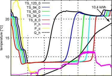
Fig. 5: Process of charging the storage down to 8 °C and discharging to 22 °C; TS_8_0 to TS_123_0 are the temperatures in the centre of the storage at heights from 8cm to 123cm; P_h is the heating power, P_c the cooling power and Q_h the integrated heat |

|
11 00:00 |
![]() лі
лі
>s
о
аз. с
ЛІ о
CL
In Figure 5 one can observe the charging and discharging process of the storage. It is cooled down (charged with cold) between 18:00 and 19:30. As a consequence of stratification the bottom part first reaches the set temperature. At 19:30 the discharging commences and the storage is heated up from the top downwards. The stratification is maintained stable as long as the slurry flow rate remains low. Higher flow rates lead to a mixing within the storage. During the entire discharging process 10,4kWh heat are absorbed by the PCS. Due to the large temperature spread (from 8 °C to 22 °C) this is only 1,3 times the amount of energy which could have been stored in water[15]. The same experiment was carried out with the storage being cooled down to different temperatures. By cooling it down to 14 °C and discharging it under the same conditions as before close to 7 kWh can be stored by the PCS. Water could have stored about 4,6 kWh in the same temperature range, so the PCS has a energy density about
1,5 times higher than water in this case. The same factor was obtained by cooling the storage down to 16 °C.
Figure 6 shows the result of the storage being cooled down to 18 °C. By heating it up to 22 °C roughly 4 kWh can be stored in it. The factor compared to water — which could store about 2,3 kWh in this temperature range — is 1,7
|
28 27 26 25 24 23 22 Q. |
|
1st International Congress on Heating, Cooling, and Buildings — 7th to 10th October, Lisbon — Portugal / |
|
21 |
|
8 |
|
00:00 |
|
05:00 |
|
06:00 |
|
time [H:M] |
|
2^ > — t—■ О (0 Cl |
|
<D |
|
Fig. 6: Process of charging the storage down to 18 °C and discharging to 22 °C, in order to cool the heating |
|
18 16 14 12 10 |
 |
circuit from 26 °C to 22 °C.
This fact implies that the use of PCS is most advisable for small temperature differences. Else the unbeatably high sensible heat capacity of water compensates the advantage of the high latent heat capacity in a narrow temperature band of the PCS.
The testing facility which is operated at Fraunhofer ISE allows the comprehensive analysis and characterization of Phase Change Slurries. Not only can the PCS be evaluated on laboratory scale or under stationary conditions — the testing facility with 500 l storage also facilitates the reproduction of reality-like applications on small scale.
The measurement of one Phase Change Emulsion demonstrates the range of parameters that can be analyzed by this facility. Also the applicability of the material under varying operation conditions is manifested. The relatively low increment in heat capacity at the large temperature band of the presented experiment confirms once more that the relative low fraction of latent storable heat argues for applications where even with water only a small temperature difference can be used. The objective for further research is therefore the development of PCS with higher melting enthalpies in a smaller temperature range. With a high AT water as a very cheap heat-carrier-fluid has clear advantages in comparison to PCS.
Acknowledgement
This paper is based on a project supported by the German Federal Ministry of Economics and Technology. Partners within the project were Fraunhofer Institute for Environmental-, Safety — and Energy Technologies (UMSICHT), IoLiTec GmbH & Co. KG and RubiTherm GmbH.
References
[1] P. Schossig, H.-M. Henning, S. Gschwander, T.. Haussmann, Micro-Encapsulated phase — change Materials integrated into constructions materials, Solar Energy Materials & Solar Cells, 2005, Vol. 89, p. 297-306, 2005
[2] Cristopia Energy Systems, Thermal Energy Storage, Product brochure, 2004
[3] Rubitherm Technologies GmbH, Rubitherm FB, Data sheet, 2006
[3] Y. Tsubota, Y. Okamoto, Prospects of Ice Slurry Systems, including PCM slurries, in Japan, IEA/ECES Annex 18 First Workshop, Tokyo, Japan, 2006
[4] H. Recknagel, E. Sprenger, Taschenbuch fur Heizung — und Klimatechnik 2005/06, Oldenbourg R. Verlag GmbH, 72nd Edition, MUnchen, Germany 2004
[5] S. Gschwander, P. Schossig; Paraffin Phase Change Slurries; 7th Conference on Phase Change Materials and Slurries for Refrigeration and Air Conditioning, Dinan, France 2006
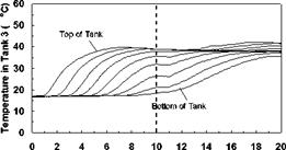
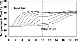
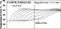
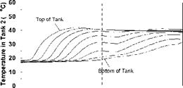
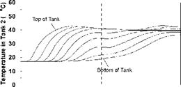
As described previously, the storage tanks were seen to stratify in a sequential manner as well as individually during the charge sequences. During periods of declining charge temperatures, there was some evidence of mixing, resulting in a slight temperature drop in the upper sections of the storage tanks. As well, it was noted that, during the intervals corresponding to low charge temperatures, the storage tanks appear to be slowly dropping in temperature. This effect is a result of a number of factors including: standby heat losses from the tank walls to the surrounding environment; heat losses from the natural convection loop; and reverse thermosyphoning caused by discharge or carry-over of heat from a high temperature storage to a lower temperature storage. A careful inspection of Figs. 8, 11 and 14 during these intervals show that the bottoms of the tanks are actually increasing in temperature as the upper sections are dropping.

|
|
||
|
|
SHAPE * MERGEFORMAT

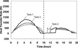
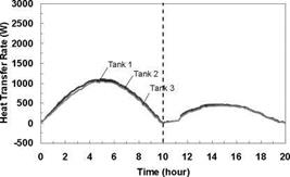
Figure 20 shows the effect of the collector loop flowrate on the magnitude of the heat transfer rate for Day 1. This figure indicates that at lower charge loop flowrates, higher degrees of stratification are obtained in the storage tanks. That is, at lower flowrates, more energy is transferred in Tank 1, driving it to a higher temperature. At higher charge loop flowrates, less energy is transferred to Tank 1 and more is carried over to Tanks 2 and 3. This result is expected as the temperatures in the storages will tend towards a uniform temperature at higher flowrates. In the extreme case, the storages will behave as though the tanks were connected in parallel. This conclusion is supported by results shown in Figs. 16 to 19
|
1st International Congress on Heating, Cooling, and Buildings, 7th to 10th October, Lisbon — Portugal / |
|
0 2 4 6 8 10 Time (hour) |
 |
 |
Fig. 20. Individual charge rates across each heat exchanger for variable input power tests at various charge flowrates.
3. Conclusion
Laboratory tests were conducted on a series-connected modular thermal storage to measure the unit’s thermal performance and temperature profiles under specified charge conditions. In particular, tests were performed to study the interaction of the individual sequentially-connected tanks and to investigate the effects of rising and falling charge loop temperatures on temperature profiles in the storage tanks. Preliminary results indicate that sequential stratification was observed for the charge profiles studied however a small amount of mixing was observed in the upper section of the storage tanks due to falling charge temperatures in the afternoon period. In addition, results indicate that a small amount of heat was also carried over from the high temperature storage to the lower temperature, downstream storages during charging. Furthermore, the dependence of the heat transfer rate on the magnitude of the charge loop flowrate was also shown. Finally as predicted by theory, as collector loop flow rate is increased, the distinction between the series and parallel connected storages disappears.
Acknowledgements
This study was supported by the Canadian Solar Buildings Research Network, the Natural Science and Engineering Research Council of Canada and EnerWorks Inc.
References
[1] Mather, D. W., Hollands, K. G. T. and Wright, J. L. 2002. Single — and Multi-tank Energy Storage for Solar Heating Systems: Fundamentals, Solar Energy 73, pp. 3-13.
[2] Cruickshank, C. A. and Harrison, S. J., 2006. Experimental Characterization of a Natural Convection Heat Exchanger for Solar Domestic Hot Water Systems, Proceedings of ISEC 2006, International Solar Energy Conference, Denver, Colorado, USA.
[3] Cruickshank, C. A. and Harrison, S. J. 2006. Simulation and Testing of Stratified Multi-tank, Thermal Storages for Solar Heating Systems, Proceedings of the Eurosun 2006 Conference. Glasgow, Scotland.
[4] Cruickshank, C. A. and Harrison, S. J. 2006. An Experimental Test Apparatus for the Evaluation of MultiTank Thermal Storage Systems, Proceedings of the Joint Conference of the Canadian Solar Buildings Research Network and Solar Energy Society of Canada Inc. (SESCI), Montreal, Quebec.
[5] Cruickshank, C. A. and Harrison, S. J. 2008. Experimental Evaluation of a Multi-tank Thermal Storage Under Variable Charge Conditions, Accepted for Publication in the Proceedings of the Joint Conference of the Canadian Solar Buildings Research Network and Solar Energy Society of Canada Inc. (SESCI). Fredericton, New Brunswick.
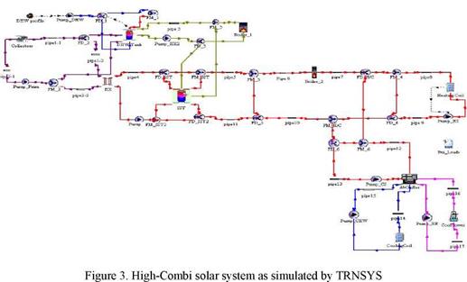
The simulations were performed using TRNSYS [TRNSYS, 2006]. The case study refers to a 700 m2 house located in Athens, Greece, with about 17 kW peak heating and 22 kW peak cooling load. The simulations were performed on a two-step approach. The first one refers to the building and estimates the heating and cooling loads. The second one refers to the entire solar system and investigates its performance, using as an input the heating and cooling loads (from the first step).
This two-step approach was implemented in order to have a faster simulation system and minimize convergence problems. The disadvantage of such an approach is that there is no dynamic interaction between the solar system and the building loads. Accordingly, it is assumed that at each time-step the system covers the total heating and cooling demand of the building. However, by monitoring the backup energy consumption (e. g. from the conventional heat source, the boiler) it is possible to determine the system’s performance in meeting the loads.
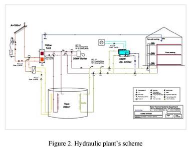
As already mentioned, one of the main objectives of this research work is to determine the most financially attractive and technically feasible configuration that approaches (or reaches) a solar fraction of 100%. The investigated configuration is illustrated in Figures 2 and 3.
|
|
|
|
This configuration is designed to cover the thermal demands for cooling, space heating and DHW. The useful energy gain collected by the solar collectors is transferred to the DHW tank (1st priority) or to the SST through an external heat exchanger (2nd priority).
When the water temperature in the DHW tank is less than the required (55 oC), then the SST provides the additional heat through an internal heat exchanger immersed on the upper part of the DHW tank. If the SST is not charged enough then the boiler is activated and heat is transferred through the same heat exchanger to the DHW tank. In heating mode, heat is removed from the SST to the floor heating circuit to meet the heating demand, while in cooling mode the heat drives the absorption chiller to produce chilled water that is fed to the fan coils to meet the cooling demand. If the stored energy in the SST is not enough to cover the heating or cooling demand, the boiler is activated to provide the supplementary energy. The difference between the hydraulic scheme and the TRNSYS deck is the use of an extra boiler in TRNSYS for simulation reasons. The main system parameters are shown in Table 1.
|
Table 1. Main characteristics of the simulated High-Combi solar system.
|
An optimization procedure has been implemented in order to define the optimum dimensioning of the solar plant. The optimization criteria was to achieve at least a total solar fraction (for cooling, heating and DHW) of 95% with the most financially attractive configuration. The variables for the parametric simulations were the collectors’ area and the SST volume, both associated with a cost function.
The resulting optimized plant configuration (180m2 collectors in combination with a 200m3 SST) has a collectors’ area that equals to about 25% of the house living area (a value that falls in the range of conventional solar combi plants collectors dimensioning). Its total solar fraction is high (95%) and the space heating fraction reaches 100%.
By reaching 100% space heating fraction and a high total fraction (95%) we can be quite certain that there is no need for an auxiliary boiler in the house under investigation[29]. In fact, a 93% solar fraction for DHW is fictitious and we can easily approach or even reach 100% in practice, using a smart system control (that has not yet been implemented in TRNSYS). According to the currently implemented system control during winter, the DHW tank will be charged by solar heat only when the collectors have reached a temperature that is higher than the DHW tank’s bottom temperature by a specified temperature difference AT = 7 K. This charging process will stop in case that the temperature difference becomes less than 3 K. During some winter days this condition is not reached often enough to ensure 100% fraction for the DHW. This is due to the fact that the collectors are charging the SST and are therefore operating at low temperatures (thus, not satisfying for some hours or days the DHW tank temperature requirements). A smart control could simply interrupt the charging process of the SST and deliver the available solar energy to the DHW[30] tank if there is a DHW load and the incident solar radiation is higher than, for example, 300 or 400 W/m2
|
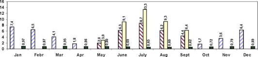
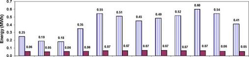
Figure 4 illustrates the monthly energy demand for the different end-uses. Energy needs
□ Qheat nQcw □ Qth_chiller ■ Qdhw |
Figure 4. Monthly energy demand for heating (Qheat), cooling (Qcw),
driving chiller (Qth_chiller) & DHW (Qdwh)
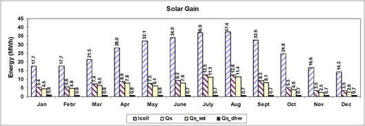
Figure 5 illustrates the main monthly system energy balance: the incident solar radiation (Icoll) and the total solar gains (Qs) with a breakdown of the energy going to the SST (Qs_sst) and to the DHW storage (Qs_dhw)
|
1st International Congress on Heating, Cooling, and Buildings^ — 7th to 10th October, Lisbon — Portugal /
Figure 5. Monthly energy balance |
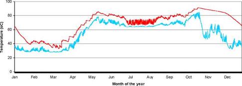
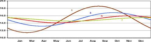
Figure 6 illustrates the SST water temperature variation over an entire year once the system is stable and shows a yearly periodic behavior.
|
Temperature of the Seasonal Storage Tank
——- TSSTTOP TSST_BOT Figure 6. Top (Tsst_top, upper line) and bottom (Tsst_bot, lower line) annual water temperature variation of the seasonal storage tank |
Charging and discharging periods are clearly distinguished on the diagram. In fact, during the first months of the year the SST is discharged (the temperature at the top drops gradually from about 65o C to under 40o C).
At about mid-March, the SST starts its charging process and its temperature increases until about mid-May. In a typical combi+ system without SST most of the available energy during spring (which is a period with low or no building energy demand) would have been lost.
During summer, the temperature fluctuations are due to continuous (practically on a daily basis) charging and discharging of the SST, since both solar radiation and cooling energy needs are available. The lowest SST temperatures occur in July; it is then again slightly charged due to the lower cooling loads.
A short but substantial charging period is identified during September — October. Once again this available energy would have been lost without the SST.
Finally, the space heating period starts at about mid-October showing an initially gradual and then sudden (towards the end of November) temperature reduction. However, a good stratification maintains relatively high top SST temperatures.
The high solar fraction is achieved mainly thanks to the SST, which maintained its seasonal role as described above, even though it has a relatively small volume. Monthly values of losses from the SST and DHW tank are illustrated in Figure 7.
1st International Congress on Heating, Cooling, and Buildings^ — 7th to 10th October, Lisbon — Portugal /
|
Thermal Losses from the Tanks
Jan Febr Mar Apr May June July Aug Sept Oct Nov Dec □ Qsst_loss □ Qdhw_loss Figure 7. Monthly thermal losses from the tanks |
Summing up the monthly values illustrated in Figure 7, the energy losses from the SST to the ambient ground are 5.0 MWh. On the other hand, the supplied energy from the SST to the heating and cooling distribution system and to the DHW tank accounts to 73.0 MWh. A good indicator for the performance of the SST is set by the fraction of the energy lost to the ambient divided by the useful energy supplied; this fraction equals to about 7% in our case. This is achieved by the good insulation installed and the position of the tank which is buried in the ground where the temperature in depths below 5 meters becomes relatively constant and equal to around 15 oC. The temperature of the ground for the climate of Athens in different depths is illustrated in Figure 8.
|
Ground Temperature variation with depth (oC)
I Tground_1m Tground_3m Tground_5m Tground_7m Figure 8. Ground Temperature in various depths for climatic conditions of Athens, Greece Comparison with alternative solutions |
The above optimized configuration (with 180 m2 of solar collectors and a SST of 200 m3) referred as plant A, is compared with two other possible configurations. An identical plant (referred as plant B) in terms of collectors’ area, hydraulics and controls, but without a SST, has been simulated. Plant B has a typical “combi” type storage size, i. e. 100 l of storage per unit solar collector area. By comparing plant A with plant B it is possible to identify the advantages and disadvantages (in energy and financial terms) of implementing a SST to a conventional combi+ plant. A similar exercise was carried out by defining a plant C that corresponds to conventional combi+ plant (without SST) but, this time, dimensioned in a way to approach the total solar fraction of plant A. This comparison reveals which of the following approaches is more suitable as we are trying to achieve high solar fractions: to increase the collector area (and proportionally the storage) or to incorporate a SST. The main results are summarized in Table 2.
|
Table 2. Main characteristics and results of plants “A” (with SST), “B” (same collectors area as “A” but no SST) and “C” (attempt to achieve similar solar fractions as in “A”).
|
Main hypotheses for economic calculations are the following:
Subsidies for solar combi+ plants: 50%; Conventional system capital cost: refers to the (electric) air cooled water chiller and the boiler ; Cost of absorption chiller : 30 000€; Inflation in conventional energy source prices (fuels and electricity): 10% ; Oil boiler efficiency: 85%; Current oil price: 0.7 €/liter; Current electricity price: 0.1 €/kWh.
T. Bauer*, D. Laing, W.-D. Steinmann, U. Kroner and R. Tamme
German Aerospace Center, Institute of Technical Thermodynamics
Pfaffenwaldring 38-40, 70569 Stuttgart, Germany.
* Corresponding Author, thomas. bauer@dlr. de
Abstract
The utilization of solar generated steam in combination with a suitable storage technology could reduce the fossil fuel dependency significantly. Selection of basic storage concepts strongly depends on the working fluid. In systems using steam as a fluid, most of the heat is
transferred at nearly constant temperature by evaporation and condensation. As a result, latent heat storage systems using phase change materials (PCMs) are suitable, since this storage concept can also operate at nearly constant temperature. The presented work covers material aspects and gives a comprehensive overview of potential organic and inorganic PCMs in the temperature range 120 to 250°C. Measurements of phase diagrams and latent heats of binary alkali nitrate/nitrite systems, previously not published are reported.
Keywords: nitrate, nitrite, phase change material, thermal energy storage, solar process heat
Thermal energy storage is a vital element in order to improve the energy efficiency of thermal processes and to utilize renewable energy source effectively. Thermal energy storage is based on three major concepts, namely: sensible and latent heat, as well as thermo-chemical storage [1]. Here, the latent heat storage concept is considered. In general, research interests include the qualification of suitable phase change materials (PCMs) and the enhancement of the poor heat transfer caused by the low thermal conductivity of the PCMs. Our ongoing research focuses on high temperature latent heat storage designs for the heat carrier steam [2]. In this storage concept, both the heat carrier fluid (water/steam) and the storage material undergo a phase change at approximately the same temperature. Depending on the steam pressure (2-40 bar), a selection of PCMs with different melting temperatures in the range 120-250°C is required [2].
This paper is directed towards the selection of PCMs in this temperature range. PCMs are classified into two major groups, namely organic and inorganic materials. A further classification criterion is the type of phase change, where melting and solidification (solid-liquid) and the rearrangement of the crystal structure in the solid phase (solid-solid) can be distinguished. Table 1 shows requirements which have to be met for the selection of PCMs, where some can be considered as fundamental and others need to be mainly considered in the design of the storage system.
The equation AH = F • Tm allows an estimation of the heat of fusion of the PCM, where AH is the heat of fusion in J/mol and Tm is the melting temperature in K. For inorganic compounds, the latent heat factor F has typical values between 20 and 50 J/(mol-K) [3]. These values may be also expressed as a multiple of the molar gas constant, e. g. 3R ~ 25 J/(mol-K). This equation shows that the heat of fusion increases with the melting temperature and that compounds with a low molar mass are favorable in terms of large heat of fusion values in J/g.
In literature a variety of PCM options has been proposed [1-9]. First organic and second inorganic PCMs will be discussed (Fig. 1 and 2).
|
Table 1. General PCM requirements.
|
The hydration reaction involves a reaction between water vapor and the dehydrated material. This reaction determines the amount of power that can be delivered to a load in a practical system and the temperature level at which the power can be delivered.
|
Fig. 5. The effect of water vapor pressure (PH2O) and temperature (T) on hydration |
 |
The first hydration experiments [8] at ECN indicated that the material was able to take up water after dehydration. Furthermore it was discovered that the layer thickness is an important factor in hydration: thick layers reduce the hydration rate considerably, indicating that the water vapor transport through the layer is the limiting factor. The experiments also suggested that the water uptake was strongly reduced when the hydration was performed at elevated temperatures and reduced water vapor pressures. To further investigate this observation, it was decided to study the effect of water vapor pressure and temperature on the hydration process for constant layer thickness. The results of these experiments are shown Figure 5:
First, the hydration was studied at 25°C and for a water vapor pressure corresponding to the practical conditions (PH2O=1.3 kPa), where a borehole at ground temperature provides the water vapor. In this case, the material slowly takes up a small amount of water (nr.1 in Figure 5). Increasing the water vapor pressure (PH2O=2.1 kPa, nr.2 in Figure 5) at 25°C, results in a larger amount of water taken up by the material, although the hydration rate is still slow. Additional experiments reveal that this large uptake of water results in the release of ~91% of 2.3 GJ/m3 (or 2.1 GJ/m3) of the energy stored during dehydration. The results presented in Figure 5 show that the hydration strongly depends on the water vapor pressure and suggest that the water vapor pressure provided by the bore hole at ground temperature may not be sufficient to release all of the energy stored during dehydration.
The effect of temperature on hydration was also investigated. A typical low-temperature domestic heating system requires >40°C for space heating. For this reason it was decided to study the hydration at 50°C at a water vapor pressure of 2.1 kPa. The result (nr.3 in Figure 5) shows that, although the water vapor pressure is almost twice the value used in a practical system (PH2O=1.3 kPa), the material is unable to take up water (and deliver heat) at 50°C. This means that the application of magnesium sulfate as thermochemical storage material is quite problematic.
The characterization of magnesium sulfate revealed that the material can be dehydrated using solar thermal collectors (<150°C). Almost 10 times more energy compared to water of the same volume can be stored using magnesium sulfate. The hydration experiments revealed that the material is also able to take up water while releasing a part of the stored energy. However, the amount of energy released during hydration depends on the temperature and the water vapor pressure. The experimental results indicate that the material cannot release all the stored heat under practical conditions, which severely limits the application of magnesium sulfate as thermochemical storage material.
Nevertheless, the characterization of magnesium sulfate gives us much needed insight in the dehydration and hydration behavior of a salt hydrate. Although the application of magnesium sulfate as TCM turns out to be quite problematic, it gives a blue-print on how to characterize salt hydrates for thermochemical heat storage. It is expected that other salt hydrates can perform better, and the characterization of magnesium sulfate is a reference point for future characterization of other salt hydrates for thermochemical seasonal heat storage.
This research was performed within the WAELS project: a cooperation between ECN, TNO, and the Eindhoven University of Technology, and partly funded by SenterNovem, an agency of the Dutch Ministry of Economic Affairs. The work on thermochemical heat storage is part of the long-term work at ECN on compact storage technologies.
[1] Visscher, K. Veldhuis, J. B.J., Oonk, H. A.J., van Ekeren, P. J. and Blok, J. G.,. (2004) ECN Report ECN-C— 04-074: Compacte chemische seizoenopslag van zonnewarmte; Eindrapportage, ECN, Petten
[2] Emons, H. H., Ziegenbalf, G., Naumann, R. and Paulik, F., Thermal decomposition of the magnesium sulfate hydrates under quasi-isothermal and quasi-isobaric conditions, J. Therm. Anal. 36, 1265-1279 (1990)
[3] Ruiz-Agudo, E., Martin-Ramos, J. D., and Rodriguez-Navarro, C., Mechanism and kinetics of dehydration of epsomite crystals formed in the presence of organic additives, J. Phys. Chem. B. 111, 41-52 (2007)
[4] Hamad, S. El D., An experimental study of salt hydrate MgSO4.7H2O, Therm. Acta 13, 409-418 (1975)
[5] Phadnis, A. B, and Deshpande, V. V., On the dehydration of MgSO4.7H2O, Therm. Acta 43, 249-250 (1981)
[6] Paulik, J., Paulik, F., and Arnold, M., Dehydration of magnesium sulfate heptahydrate investigated by quasi isothermal-quasi isobaric TG, Therm. Acta 50, 105-110 (1981)
[7] Van der Voort, I. M., Characterization of a thermal chemical material storage, Eindhoven University of Technology, 2007
[8] Zondag, H., Essen, V. M. van, He, Z., Schuitema, R. and Helden, W. van, Characterization of MgSO4 for thermochemical storage, in Second International Renewable Energy Storage Conference (IRES II), Bonn, Germany (2007)
This study assumes a prototype greenhouse with floor dimensions of 10m x 30m and total glazed area — roof and walls — of approximately 600 m2 made from structured polycarbonate (PP) sheets. This material was chosen due to its thermal isolation properties (U = 3,4 W/m2°C [2]), mechanical stability and weight characteristics. For a AT of 15°C, i. e., considering a minimum inside temperature of 14°C and a minimum outside temperature of -1°C, the thermal loss associated with the greenhouse surface is (equation 1):
Q = U x A x AT = 3,4 x 600 x 15 = 30,6 kW (1)
where Q also represents the power of the required auxiliary heating system that should be installed.
Previous calculation considers that all air inside this greenhouse is heated through convectors with forced circulation. Therefore, all air in contact with the glaze will also be at the temperature required by the crops.
The procedure to determine the design load of a greenhouse heating system (i. e., "sizing" the boiler) is different from the procedure to determine the projected operational heat demand and subsequent fuel consumption during any given day (or entire heating season). The selection of the size of the boiler is primarily dependent upon the greenhouse surface area, insulation properties, and the maximum expected difference of the inside set point air temperature from the minimum expected outside air temperature. This calculation represents the design condition for the worst — case situation. However, the real operating costs to heat the greenhouse are dependent on the difference of the actual inside and outside air temperatures at each and every moment of the heating season, and the length of time that each of those temperature conditions occurs. Thus, the design heating load capacity of the boiler may rarely (or never) be reached, but the boiler must provide heat at some level, which is less than the design capacity, nearly all the time during the heating season.
Unless the air temperature difference is known on an hourly basis through historical weather data or by real time data acquisition system, the Degree Day Procedure can be used to determine the amount of heat that will be needed over a given period [3].
The difference between the minimum acceptable temperature inside the greenhouse (ex. 14°C) and the outside air temperature, multiplied by the number of the hours in a day and by the number of the days in that month, will give us the total Degrees Month to be used in the equation of the thermal losses. This procedure assumes that there is no daily energy gain from solar radiation and that the inside to outside air temperature difference is the same for the entire 24-hour period.
Degrees Month = (Reference temperature — Average month temperature) x 24 hours x nr. of days in that month;
Average monthly consumption on this 300 m2 greenhouse example can thus be estimated. Annual total will be 32.063,9 kWh or, with a 90% efficiency, around 3.281 liters of diesel (1 liter of diesel ~ 10,75 kWh [4])
Separation in two solid phases on freezing could be expected for binary eutectics compounds, but the specific arrangement of the two phases in the solid is unknown. The problem is more complexly exciting when the sample is a composite, elaborated by graphite and an inorganic salt.
Energy dispersive x-ray microanalysis (EDS) based on scanning electron microscopy (SEM), SEM/EDS, allowed the observation in depths of 1-2 microns. The backscattered electrons, emitted from the depth of a sample illustrated readily the chemical phase difference between particles and the composite (BEI image, red pointer, Table 4.). Evidently, some small crystallites of single K and Na components of the salt avoided the melting process and formed solidified mechanical mixtures.
RSiC-walls were tested in the heat exchanger with different porosities, pore sizes and basic structures, including solid material and a channelled structure. The channelled walls, cut as slices from diesel particulate filters, appear appropriate due to their small wall thickness and high open porosity of 45 %. Additionally, they provide a cleaning option against clogging by applying pressure from the channels. However, wall cracks were detected after short operation time, which are attributed to the pressure forces on the walls coinciding with strains of the clamping. The solid walls with porosity of 25 % disposed of excellent mechanical strength at the cost of extreme pressure drop and were not used for this reason.
In view of the project deadline further experimental work was focussed on the heat transfer analysis. To realize principle operation the ceramic walls were replaced by temperature resistant steel screens with thermal strength up to 1300 °C.
1.3. Design Criteria
After the initial study of the authors [6], it was hoped that an examination of alternative STTS designs would help to better characterize the charging performance of the current STTS concept. It would also serve as a proving ground for the Exergy Charge Response index. As we wished to maintain the external shape of the STTSs, the study also holds specific bearing to the optimal design of large horizontal thermal energy stores.
1.4. New Concepts
|
Figure 2. Original Concept (Tank 1) Figure 3. Repositioning of Inlet Figure 4. Removal of Center Baffle and Outlet Ports (Tank 2) (Tank 3) |
 |
Seven concepts of the STTSs are presented and studied in this work, including the original design. These are illustrated below in Figures 2 to 8, showing cross-sectional views of each design.
|
Figure 5. Addition of Upper and Lower Baffles (Tank 4) |
|
Figure 6. Addition of Second Inlet Port (Tank 5) |
 The first four new concepts (Figures 3 to 6) were developed from sequential changes made to the original STTS (Figure 2). The continued usage of the large horizontal baffles has both practical and analytical benefits. Not only are they simple to implement physically, the reduced meshing complexity of the baffled tanks allows for increased confidence in the validity of the CFD analysis carried throughout.
|
Figure 7. Horizontally Partitioned STTS (Tank 6) |
|
Figure 8. Horizontally Partitioned STTS with Slotted Plenums (Tank 7) |
 |
 |
The use of large horizontal baffles to encourage thermal stratification in thermal energy stores has been examined elsewhere [2], and has proven to serve useful particularly for vertical tanks, where the inlet/outlet flows are parallel to the direction of stratification. For Tanks 4 and 5, the purpose of the baffles is to allow the velocity of the inlet fluid to reduce significantly before coming into to contact with the larger region of the tank, thereby minimizing thermal mixing.
Figures 7 and 8 illustrate a different configuration altogether, using vertical baffles to horizontally partition the STTS into four nodes. Tank 7 also incorporates a slotted plenum at the inlet region to reduce turbulent mixing caused by the initial jet plumes. The designs were created principally from qualitative objectives, without a particular design guide for horizontally partitioned thermal energy stores. A more concrete study of such systems is under research at Shanghai Jiao Tong University [9].
Figure 5 shows a tube covered with an ice layer. The media temperature in the tube is lower than the temperature in the ice layer and the surrounding liquid phase. Basically solidification Processes can be described mathematically with the following equations assuming quasi-stationary conditions [3].
|
= X * A * cond ice ice |
|
Qlt = Ah * m = p. * Ah lat s ice ice s |
|
Figure 8: Tube with ice layer |
|
Q cond Q lat + Q con The conducted heat flow rate is calculated |
|
33 dr |
|
ice |
|
dVic |
|
dt |
|
(1) (2) (3) |
|
ice |
|
The equation for the latent heat fraction is |
|
r |
|
Q |
The heat balance at the ice layer surface was calculated with equation (1)
The convective heat fraction was calculated with equation (4)
|
(4) |
![]() Qcon =aout * Aice *(^-^s )
Qcon =aout * Aice *(^-^s )
The rate of increase in the volume of solid ice is calculated from
d V. dr
ice _ 2* r * n *L * lce
dt dt
Substituting Equation (2), (3), (4) and (5) in Equation (1) yields
|
t *9* tt^-T * ice, sol ‘ Tube ice |
|
aout *2*n* LTube * rice *(Soo — Ss ) +Pice * Ahs *2*n* L |
|
dric |
|
ice |
|
Tube ice |
|
dt |
|
dS |
|
r ice |
|
(6) |
|
|
SHAPE * MERGEFORMAT
