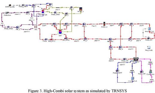
The simulations were performed using TRNSYS [TRNSYS, 2006]. The case study refers to a 700 m2 house located in Athens, Greece, with about 17 kW peak heating and 22 kW peak cooling load. The simulations were performed on a two-step approach. The first one refers to the building and estimates the heating and cooling loads. The second one refers to the entire solar system and investigates its performance, using as an input the heating and cooling loads (from the first step).

This two-step approach was implemented in order to have a faster simulation system and minimize convergence problems. The disadvantage of such an approach is that there is no dynamic interaction between the solar system and the building loads. Accordingly, it is assumed that at each time-step the system covers the total heating and cooling demand of the building. However, by monitoring the backup energy consumption (e. g. from the conventional heat source, the boiler) it is possible to determine the system’s performance in meeting the loads.

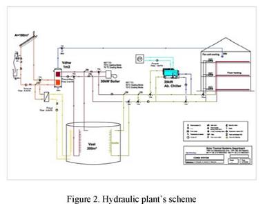
As already mentioned, one of the main objectives of this research work is to determine the most financially attractive and technically feasible configuration that approaches (or reaches) a solar fraction of 100%. The investigated configuration is illustrated in Figures 2 and 3.

This configuration is designed to cover the thermal demands for cooling, space heating and DHW. The useful energy gain collected by the solar collectors is transferred to the DHW tank (1st priority) or to the SST through an external heat exchanger (2nd priority).

When the water temperature in the DHW tank is less than the required (55 oC), then the SST provides the additional heat through an internal heat exchanger immersed on the upper part of the DHW tank. If the SST is not charged enough then the boiler is activated and heat is transferred through the same heat exchanger to the DHW tank. In heating mode, heat is removed from the SST to the floor heating circuit to meet the heating demand, while in cooling mode the heat drives the absorption chiller to produce chilled water that is fed to the fan coils to meet the cooling demand. If the stored energy in the SST is not enough to cover the heating or cooling demand, the boiler is activated to provide the supplementary energy. The difference between the hydraulic scheme and the TRNSYS deck is the use of an extra boiler in TRNSYS for simulation reasons. The main system parameters are shown in Table 1.

Table 1. Main characteristics of the simulated High-Combi solar system. Collector field 180 m2 Primary circuit fluid Mixture of propylene glycol (30%) and water Primary circuit flow 5.4 m3/h (30l/h per m2 of collectors’ area) Heat exchanger coefficient 10 kW/K Corresponding heat exchanger LMTD 5 K DHW storage tank 1 m3 Seasonal Storage Tank (SST) 200 m3 Back-up heater 30 kW Chiller type Absorption Chiller power 35 kW Cooling tower power 85 kW Chiller input flow 3.5 m3/h Recooling flow 12 m3/h Maximum heating flow 3.5 m3/h (variable flow depending on load) Maximum cooling flow 4.3 m3/h (variable flow depending on load) Heating supply/return temperature 33/28°C Cooling supply/return temperature 7/12°C Maximum heating load 16.7 kW Building’s living area 700 m2 Annual heating energy demand 31.6 MWh (45 kWh/m2) Maximum cooling load 21.6 kW Annual cooling energy demand 27.6 MWh (40 kWh/m2) Annual DHW energy demand 9.2 MWh

An optimization procedure has been implemented in order to define the optimum dimensioning of the solar plant. The optimization criteria was to achieve at least a total solar fraction (for cooling, heating and DHW) of 95% with the most financially attractive configuration. The variables for the parametric simulations were the collectors’ area and the SST volume, both associated with a cost function.

The resulting optimized plant configuration (180m2 collectors in combination with a 200m3 SST) has a collectors’ area that equals to about 25% of the house living area (a value that falls in the range of conventional solar combi plants collectors dimensioning). Its total solar fraction is high (95%) and the space heating fraction reaches 100%.

By reaching 100% space heating fraction and a high total fraction (95%) we can be quite certain that there is no need for an auxiliary boiler in the house under investigation[29]. In fact, a 93% solar fraction for DHW is fictitious and we can easily approach or even reach 100% in practice, using a smart system control (that has not yet been implemented in TRNSYS). According to the currently implemented system control during winter, the DHW tank will be charged by solar heat only when the collectors have reached a temperature that is higher than the DHW tank’s bottom temperature by a specified temperature difference AT = 7 K. This charging process will stop in case that the temperature difference becomes less than 3 K. During some winter days this condition is not reached often enough to ensure 100% fraction for the DHW. This is due to the fact that the collectors are charging the SST and are therefore operating at low temperatures (thus, not satisfying for some hours or days the DHW tank temperature requirements). A smart control could simply interrupt the charging process of the SST and deliver the available solar energy to the DHW[30] tank if there is a DHW load and the incident solar radiation is higher than, for example, 300 or 400 W/m2

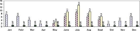
Figure 4 illustrates the monthly energy demand for the different end-uses. Energy needs □ Qheat nQcw □ Qth_chiller ■ Qdhw

Figure 4. Monthly energy demand for heating (Qheat), cooling (Qcw),
driving chiller (Qth_chiller) & DHW (Qdwh)

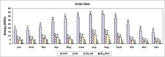
Figure 5 illustrates the main monthly system energy balance: the incident solar radiation (Icoll) and the total solar gains (Qs) with a breakdown of the energy going to the SST (Qs_sst) and to the DHW storage (Qs_dhw)

1st International Congress on Heating, Cooling, and Buildings^ — 7th to 10th October, Lisbon — Portugal / Figure 5. Monthly energy balance

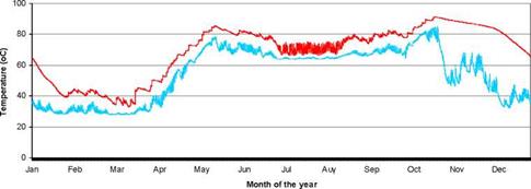
Figure 6 illustrates the SST water temperature variation over an entire year once the system is stable and shows a yearly periodic behavior.

Temperature of the Seasonal Storage Tank ——- TSSTTOP TSST_BOT Figure 6. Top (Tsst_top, upper line) and bottom (Tsst_bot, lower line) annual water temperature variation of the seasonal storage tank

Charging and discharging periods are clearly distinguished on the diagram. In fact, during the first months of the year the SST is discharged (the temperature at the top drops gradually from about 65o C to under 40o C).

At about mid-March, the SST starts its charging process and its temperature increases until about mid-May. In a typical combi+ system without SST most of the available energy during spring (which is a period with low or no building energy demand) would have been lost.

During summer, the temperature fluctuations are due to continuous (practically on a daily basis) charging and discharging of the SST, since both solar radiation and cooling energy needs are available. The lowest SST temperatures occur in July; it is then again slightly charged due to the lower cooling loads.

A short but substantial charging period is identified during September — October. Once again this available energy would have been lost without the SST.

Finally, the space heating period starts at about mid-October showing an initially gradual and then sudden (towards the end of November) temperature reduction. However, a good stratification maintains relatively high top SST temperatures.

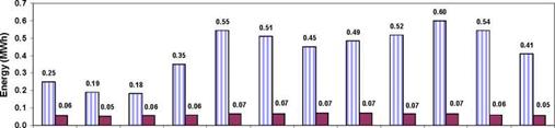
The high solar fraction is achieved mainly thanks to the SST, which maintained its seasonal role as described above, even though it has a relatively small volume. Monthly values of losses from the SST and DHW tank are illustrated in Figure 7.

1st International Congress on Heating, Cooling, and Buildings^ — 7th to 10th October, Lisbon — Portugal /

Thermal Losses from the Tanks Jan Febr Mar Apr May June July Aug Sept Oct Nov Dec □ Qsst_loss □ Qdhw_loss Figure 7. Monthly thermal losses from the tanks

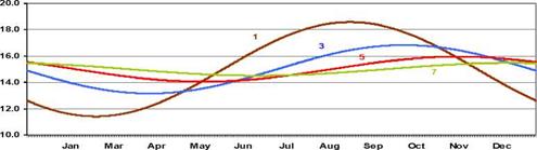
Summing up the monthly values illustrated in Figure 7, the energy losses from the SST to the ambient ground are 5.0 MWh. On the other hand, the supplied energy from the SST to the heating and cooling distribution system and to the DHW tank accounts to 73.0 MWh. A good indicator for the performance of the SST is set by the fraction of the energy lost to the ambient divided by the useful energy supplied; this fraction equals to about 7% in our case. This is achieved by the good insulation installed and the position of the tank which is buried in the ground where the temperature in depths below 5 meters becomes relatively constant and equal to around 15 oC. The temperature of the ground for the climate of Athens in different depths is illustrated in Figure 8.

Ground Temperature variation with depth (oC) I Tground_1m Tground_3m Tground_5m Tground_7m Figure 8. Ground Temperature in various depths for climatic conditions of Athens, Greece Comparison with alternative solutions

The above optimized configuration (with 180 m2 of solar collectors and a SST of 200 m3) referred as plant A, is compared with two other possible configurations. An identical plant (referred as plant B) in terms of collectors’ area, hydraulics and controls, but without a SST, has been simulated. Plant B has a typical “combi” type storage size, i. e. 100 l of storage per unit solar collector area. By comparing plant A with plant B it is possible to identify the advantages and disadvantages (in energy and financial terms) of implementing a SST to a conventional combi+ plant. A similar exercise was carried out by defining a plant C that corresponds to conventional combi+ plant (without SST) but, this time, dimensioned in a way to approach the total solar fraction of plant A. This comparison reveals which of the following approaches is more suitable as we are trying to achieve high solar fractions: to increase the collector area (and proportionally the storage) or to incorporate a SST. The main results are summarized in Table 2.

Table 2. Main characteristics and results of plants “A” (with SST), “B” (same collectors area as “A” but no SST) and “C” (attempt to achieve similar solar fractions as in “A”). Plant Collectors Area (m2) Storage Volume (m3) Total Solar Fraction (f) Heating Solar Fraction (fh) Cooling Solar Fraction (fc) Capital Cost (€) Annual Operat. Costs (€) Pay­ Back time (y) A (with SST) 180 200 95% 100% 92% 184 00 0 827 11,7 B (no SST) 180 18 79% 72% 82% 100 000 1491 8,5 C (same “Я 360 36 99% 98% 100% 163 000 865 11,0 Convent ional — — 0% 0% 0% 13 000 4845 —

Main hypotheses for economic calculations are the following:

Subsidies for solar combi+ plants: 50%; Conventional system capital cost: refers to the (electric) air cooled water chiller and the boiler ; Cost of absorption chiller : 30 000€; Inflation in conventional energy source prices (fuels and electricity): 10% ; Oil boiler efficiency: 85%; Current oil price: 0.7 €/liter; Current electricity price: 0.1 €/kWh.