An important design specification for a TCM system is the required thermal power input, which is related to the amount of material in the reactor and how fast the solar heat can be fed to the material. Typically, this process is complicated by the low thermal bed conductivity of the TCM powder, which is due to the low conductivity of the gas in the pores between the particles. Also the water vapour transport out of the layer of TCM powder is critical, and insufficient vapour transport out of the material may result in unwanted melting. One can try to improve the heat and vapour transfer simultaneously by stirring, thereby speeding up the conversion. Three design cases have been evaluated for dehydration reactor volume in the following paragraphs, under the assumptions that the reactor power required is 3 kW (see Fig 4) and that heat transport is the limiting factor.

4.1 TCM fluidised bed reactor

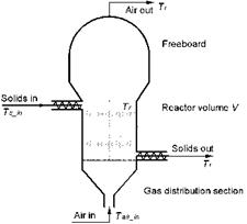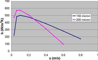
A fluidised bed reactor (see Fig. 5a) creates very good mixing of the powder, thereby improving strongly the vapour transport and the heat transfer. Fig. 5b shows that for small particles, the fluidisation velocity is small, limiting the power required for the fluidisation, while the heat transfer to the embedded heat exchanger is strongly increased. However, the fluidisation may cause breakup of TCM particles that are fragile already due to the cracks caused by repetitive hydration and dehydration. The resulting fine dust may be blown out of the fluidised bed reactor, thereby reducing the amount of active material. Also, this very fine powder cannot be fluidised properly.

For the case of dehydration of the TCM in a 3 kW reactor, assuming 200 micron particles and an effective heat transfer of about 350 W/m2K to the immersed plate heat exchanger (consisting of 11 parallel plates of 7.5 cm x 19 cm each), this would lead to a reactor fluidisation section (excluding the freeboard and the gas distribution section) of about 20 cm in length and 11 cm diameter, in which about 40% of the open volume would be filled with TCM, while about 30% of the reactor volume is taken up by the heat exchanger volume. Due to the low fluidisation velocity (resulting from the small particle size), the power required for fluidisation is in the order of a few Watt. This seems promisingly low, provided that the pressure drop in the porous support and other parts of the reactor can also be kept small.

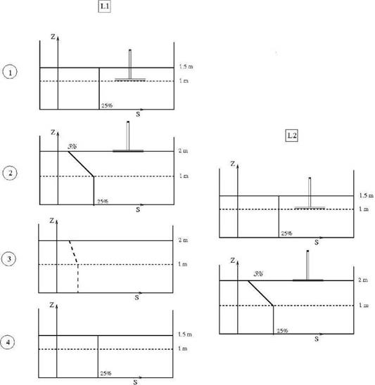
If the Aquaculture plant is build near marine salt works the DSP could be a good alternative to a conventional Solar Pond. We are going to considered two typical side-by-side salt works with 1000 m2 surface and 2m depth represented by L1 and L2 (Figure 5).

The first basin is constructed in order to act as a Solar Pond (Figure 5:1) and will work in a regime adjusted to aquaculture operation with an energy extraction of 30 kW. The only operation to be done is to create the gradient in L1 (Figure 5:2).

This is usually done with a diffuser that fills the pond from 1.5 m to 2 m depth. Here a salinity gradient is created being upper zone with 3% (seawater salinity) and the bottom with 25% of salt concentration. This operation takes about one week. At this time L2 basin is in a stand by mode.

If we only consider losses by salt diffusion L1 can work for a long time (about nine years) (Figure 5:3). After this the NCZ of L1 will be homogenized (Figure 5:4). Nevertheless there are other kinds of instabilities that accelerate this process. On the other hand we need to alternate the operation of L1 and L2 ponds with a periodicity of one year.

When L2 begins to be constructed as a Solar Pond (Figure 5:2a) L1 can aid to raise the initial temperature by energy extraction transfer. After about one week L2 is in conditions to work (Figure 5:2b). In this way L1 and L2 are connected.

If L1 is not completed homogenized (Figure 5:4) the process must be accelerated. There are several processes to do this. Nevertheless, the simpler one is to stop the heat extraction. This will quickly raise the temperatures at the SZ and will destabilize the pond (Figure 6).

After this stage is reached, one must regain the initial concentration of 25% at the bottom. The remaining water must be evaporated from the pond until this concentration is reached. Basic calculations give the rate of evaporation to reach the original salt concentration of 25%. Results points that we need 51 days for a pond temperature of 40 °С, 29 days for 50 °С, and only 10 days for 80°C.

2. — Conclusions

We may conclude that for Aquaculture facilities these kind of solar ponds, are well designed and considerable less expensive than conventional ones. We must emphasize that this concept needs an annual periodicity of construction that is the periodicity of marine salt works recovering. In this way we have always a Pond that is working. The key of the concept of Dual Pond is to standardized maintenance operations with an annual periodicity.

The results here presented are a first approximation and more work must be done to deal the concept with assurance. Nevertheless in a first insight it seems to work giving the thermal energy needed for the application in mind.

References

[1] — M. R. Jaefarzadeh, A. Akbarzadeh, "A mechanism for layer formation in a double diffusive fluid", Solar Energy, Vol. 73, (5), pp:375-384, 2002

[2] — T. Radko, "A mechanism for layer formation in a double diffusive fluid", Journ. of Fluid Mechanics, 497, pp:365-380, 2003

[3] — S. Grossman, D. Lohse, "On geometry effects in Rayleigh-Benard convection", Journ. of Fluid Mechanics, 486, pp: 105-114, 2003

[4] — M. Ouni and A. Guizani, H. Lu and A. Belghith, "Simulation of the control of a salt gradient solar pond in the south of Tunisia", Solar Energy, Vol.75, pp:95-101, 2003

[5] — S. A. Enein, A. A. E. Sabaii, M. R.I Ramadan, and A. M.Khallaf, "Parametric study of a shallow solar pond under the batch mode of heat extraction", Journ. of Applied Energy, Vol.78, (2), pp:159-177, 2004

[6] — C. Angeli and E. Leonardi, “A one-dimensional numerical study of the salt diffusion in a salinity-gradient solar pond", Int. J. Heat and Mass Transfer, 47,pp:1-10, 2004

[7] — A. Joyce. Lagos Solares: contribuigao para o desenvolvimento de uma tecnologia. PhD thesis, U. N.L.1992

[8] — H. Weinberger, " The Physics of the solar pond", Solar Energy,8, 2, 1964

[9] — F. Zangrando /’Technical Note-Simple method for establish salt gradient solar ponds", Solar Energy, 24, pp:467-470, 1980.

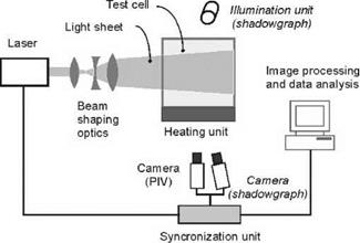
The experiments are carried out in a box with a square base of 100×100 mm and a height of 150mm. The base of the test cell is made of copper with 5 mm thickness and the lateral sidewalls are made in 4 mm transparent acrylic. The sidewalls are isolated by 30 mm polystyrene coated with 5 mm ceramic fiber. This isolation is removed temporarily each time flow visualization with PIV and Shadowgraph techniques occurs. A precision heater is used to provide uniform heating over the base of the copper test cell at a prescribed temperature. The desired linear salinity gradients are created using the two tanks method described by Oster [9] and Hill [10].

By applying the PIV system the measurement of velocities in the convective regions and the observation of the flow patterns are accomplished. Figure 1 shows the PIV setup. A 10Hz Nd:YAG Q-switched laser with frequency doubled 532 nm wavelength emits a circular light beam, and an optical setup (beam shaping optics) creates a sheet of light with 1 mm thickness and low divergence height. This sheet of light crosses the inspected volume and the light scattered by the seeding particles is visualized by a CCD camera, perpendicular to the light sheet. The seeding particles, hollow glass spheres with an average diameter of 12 pm, are mixed in the aqueous salt (NaCl) solutions before the formation of the stratified layer. The synchronization between the laser and the camera is made by an electronic circuit developed for that purpose. For each PIV acquisition 30 images of particles, exposed to individual frame and with an acquisition rate of 10Hz, are captured. Afterwards, these images are processed using specific software (Dynamic. Studio from Dantec Dynamics A/S). The processing consists in the cross-correlation of each pair of images of particles captured, producing a vector map of the instantaneous velocity field of the field of view. At present study, the field of view of the PIV system is a rectangle with 64 mm height and 84 mm width.

Figure 1 also includes the schematic of the Shadowgraph setup. This method makes use of a 100W halogen lamp that projects the emitted light on a semi-transparent screen placed near the test cell. This allows a near to 1:1 relation between the object and the projected shadowgraph image. Using this technique the positions of the interface zones can be identified, and their evolution analyzed. The shadowgraphs images that capture the sudden changes on the medium refractive index are visualized by a CCD camera, alternating with the PIV analysis. Both the CCD cameras have 640×480 pixels and 8.6×8.3 pm pixel pitch.

The vertical temperature and concentration of salt distributions near the centre of the test cell are measured during the experiments with a Micro Scale Conductivity and Temperature Instrument, MSCTI (from Precision Measurement Engineering, Inc) [11]. From time to time, this probe, with high special resolution (1 mm) and fast response, is made to move slowly through the system, using a computer controlled linear translation axis to command the step movement of the MSCTI and the translation velocity. The measurements were performed with a 1 mm step and with a velocity translation of 0.1 mm/s, or 0.05 mm/s. Empirical equations are used to convert conductivity data, at a giving temperature measured simultaneously, to salt concentration [12]. A vertical temperature probe rake, consisting of 16 calibrates Pt100 probes mounted at approximately 5 mm intervals, allowed the continuous measurement of the evolution of the vertical temperature profile during the experiments.

The focus of this work was the identification of suitable PCMs in the temperature range 120 to 250°C. First, literature of organic PCMs in this temperature range was reviewed. In summary, it can be pointed out that the long-term thermal stability, the reactivity with air oxygen and the high vapour pressure of organic materials are the major critical aspects. All discussed organic PCMs require hermetically sealed storage systems and this can be considered disadvantageous.

The thermal stability of inorganic materials is typically higher. Besides long-term stability, PCM selected for the steam storage application need to fulfill other requirements such as suitable properties regarding handling and economics. Another aspect is that the entire temperature range 120 to 250°C should be covered with different melting temperatures. Taking these aspects into account, the combination of two alkali nitrate/nitrites to form binary systems is a suitable option. This work selected three alkali metal nitrates (LiNO3, NaNO3, KNO3), two alkaline earth nitrates (Sr(NO3)2, Ba(NO3)2) and two alkali metal nitrites (NaNO2, KNO2). Ternary systems, such as the system KNO3-NaNO2-NaNO3, which offer a further potential but also some complexity were not considered. For the considered seven alkali nitrate/nitrites, the minimum melting temperature of all binary combinations was identified either from secondary literature or through measurements presented in this work (Table 4). It can be concluded that the considered temperature range 120 to
250°C can be covered by these systems with a maximum temperature gap of 20°C (Fig. 5). Known values of the latent heat factors were in a range from 14 to 33 J/(mol K), where LiNO3 systems had exceptionally high values of 36 and 43 J/(mol K). In this work unknown minimum melting temperatures and systems around 170°C were assessed in more detail by phase diagram determinations and melting enthalpy measurements. Although KNO2 can be regarded as an less ideal candidate material, because it is a uncommon substance and strongly hygroscopic, it is the only material of the selected candidates, which forms binary systems with a melting temperature in the range 150 to 190°C. Of the two candidates at around 170°C, KNO2-Sr(NO3)2 has been identified as the favorable system due to its higher melting enthalpy and flatter liquidus line rather than KNO2-Ba(NO3)2.

It can be pointed out that the knowledge about the binary systems varies widely. For some systems essential values such as the eutectic temperature, composition and enthalpy are unknown. The characterization of other systems has progressed much further due to their application as heat transfer carrier, salt bath fluids and molten sensible heat storage media. Examples are the KNO3- NaNO3 and KNO3-LiNO3 systems, where work on aspects such as thermophysical properties, thermal stability and steel corrosion has been reported. Hence, after the selection of PCM with a suitable melting temperature, reported in this work, full qualification of PCMs for

References

[1] H. P. Garg et al. (1985) Solar Thermal Energy Storage, Reidel Publishing.

[2] R. Tamme et al., International Journal of Energy Research, 32 (2008) 264-271.

[3] D. Steiner et al. (1982) University of Stuttgart, Rep. BMFT-FB-T 82-105. (in German)

[4] G. J. Janz et al. (1978-1981) NSRDS-NBS 61 Part I, II and IV.

[5] M. Kamimoto et al., Solar Energy, 24 (1980) 581-587

[6] B. Zalba et al., Applied Thermal Engineering, 23, (2003) 251-283.

[7] A. Hoshi, D. R. Mills, A. Bittar, T. S. Saitoh, Solar Energy 79 (2005) 332-339.

[8] C. E. Birchenall, et al., Metallurgical and Materials Transactions A, 11 (1980) 1415-1420.

[9] H. Kakiuchi (1998) IEA Annex 10, 2nd Workshop, Sofia, Bulgaria (1998).

[10] D. Chandra et al., Z. Phys. Chem., 216 (2002) 1433-1444.

[11] S. D. Sharma et al., International Journal of Green Energy, 2 (2005) 1-56.

[12] T. Ozawa et al., Thermochimica Acta, 92 (1985) 27-38.

[13] Ullmann’s Encyclopedia of Industrial Chemistry (1998), 6. Edition, Wiley.

[14] J. Font et al., Journal of material chemistry, 5 (1995) 1137-1140.

[15] R. Sakamoto et al., Thermochimica Acta, 71 (1984) 241-249.

[16] I. O. Salyer et al., Journal of Applied Polymer Science, 28 (1983) 2903 — 2924.

[17] T. Clauhen et al., Symp. 8. Internationales Sonnenforum ’92 (in German)(1992), 1259-1264.

[18] H. Inhaba et al. Transactions of the Japan Society of Mechanical Engineers. B, 63 (1997) 3382-3389.

[19] Y. Takahashi et al., Thermochimica Acta, 50 (1981) 31-39.

[20] T. Ozawa et al. (2003) Chp. 7: Energy storage, in Handbook of Thermal Analysis and Calorimetry, 2.

[21] P. A.E. Vallejo et al., Proc. of the COMSOL Multiphysics User’s Conference, Boston (2005).

[22] G. Hakvoort et al., Journal of Thermal Analysi and Calorimetry, 69 (2002) 333-338.

[23] D. G. Lovering (1982) Molten salt technology, Plenum Press.

[24] A. Verma et al., Canadian Journal of Chemical Engineering, 56 (1978) 396-398.

[25] R. P. Tye et al., Proc. 7th Symposium on Thermophysical Properties, ASME, (1977) 189-197.

[26] Y. Takahashi et al., Thermochimica Acta, 123 (1988) 233-245.

[27] Y. Abe et al., Proc. 23rd. Intersoc. Energy Conv. Eng. Conf., Denver, 2, (1988) 159-164.

[28] R. J. Calkins et al., Report SAND-81-8184, Sandia Lab. (1981).

[29] Y. Takahashi et al., Thermochimica Acta, 121 (1987) 193-202.

[30] Y. Takahashi et al., International Journal of Thermophysics, 9 (1988) 1081-1090.

[31] I. Barin (1995) Thermochemical Data of Pure Substances, 3. Edition, VCH.

[32] K. H. Stern, J. Phys. Chem. Ref. Data, 1 (1972) 747-772.

[33] R. P. Shisholina et al., Russian Journal of Inorganic Chemistry, 8 (1963) 1436-1438.

[34] E. Thilo et al., Proc. 7th. Conf. on the Silicate Industry, Hungary (1963) 79-85.

[35] M. V. Tokareva et al., Zhurnal Neorganicheskoi Khimii, 1 (1956) 2570-2576.

[36] E. Schumann et al., Berichte der Bunsen-Gesellschaft (in German), 74 (1970) 462-470.

[37] E. M. Levin et al. (1956) Phase Diagrams for Ceramists, The American Ceramic Society.

[38] J. Alexander et al., Industrial & Engineering Chemistry, 39 (1947) 1044-1049.

[39] X. Zhang et al., Thermochimica Acta, 385, (2002) 81-84.

[40] R. W. Berg et al., Dalton Transactions (2004) 2224-2229.

[41] R. N. Grugel et al., J. Material Science Letters 13 (1994) 1419-1421.

[42] P. I. Protsenko et al., Russian Journal of Inorganic Chemistry, 6 (1961) 850-854.

[43] P. I. Protsenko et al., Russian Journal of Inorganic Chemistry, 20 ( 1975) 924-927.

Four simulation studies were performed in Subtask C. Three of them were using more or less the reference conditions defined in Subtask A [3]. One of them dealt with a complete different application to reduce boiler cycling by introducing a PCM store.

The simulation results from HEIG-VD in Yverdon-les-Bains, Switzerland concerning the advantage of macroencapsulated PCM in solar combisystems are shown in Fig. 2 [4]. It should be

reminded that the proposed system has been analysed only from the simulation side, where a water tank storage filled only with water or filled with water + PCM (paraffin RT35) is compared.

To evaluate the impact of the PCM on the performances, it is possible to define the energy gain between the Fsav, therm for the tank with PCM (Fsav, therm(W+PCM)) and only with water (Fsav, therm(W)). If this gain is higher than 0, then the PCM brings an advantage. As it can be seen in Figure 3, the gain due to using PCM is low. A decrease of the RATIO according to the increase of the Fsav, therm can also be noticed. But it should be remembered, that when the Fsav, therm is high, the solar installation is oversized. As it can be seen, adding a PCM becomes less interesting when the solar system is oversized. This is due to the fact, that when oversized, the storage of heating is less relevant.

The fractional thermal energy savings fsav, therm are a measure of the percentage of the auxiliary (non-solar) energy input for heating that can be reduced by the solar system. This term does not account for electricity use unless it is used directly for heating. The efficiency of electricity production and distribution pel is 0.4 in all cases. Hereby Qboiler and Qelheater are the energy inputs of the solar combisystem with respective efficiencies pboiler and pel. Qboiler, ref defines the energy input of a boiler of a defined conventional heating system with an efficiency of nboiler, ref [3].

Qboiler __ Qel, heater

fm>er. = 1 — —( (Equation 1)

boiler, ref

According to the additional cost of adding the PCM and the environmental impacts results described in [2], this system with PCM does not show a substantial benefit compare to a storage tank filled only with water.

Only the long term heat storage with subcooled liquid PCM (BYG DTU, Department of Civil Engineering, Denmark, Fig. 3 [5]) shows the possibility to achieve 100 % solar fraction with PCM store volumes of about 10 m3 for a 135 m2 floor area passive houses (15 kWh/m2a space heating energy demand). Water stores have to be far bigger to achieve the 100 % solar fraction. 80 — 90 %

solar fraction can be achieved also with water stores of 5 — 10 m3. Taking into account the long term heat losses of water stores the size reduction is far bigger.

At the Institute of Thermal Engineering (IWT), Graz University of Technology, Austria different hydraulic systems were investigated in terms of their ability to reduce boiler cycling operation [6]. In the following a description of the hydraulic systems, which are used in the simulations, is given. Table 2 shows a summary of all simulated concepts.

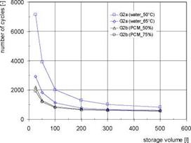
The results for the system with water storage (G2a) and for systems with water storage with integrated PCM modules (G2b) are shown in Fig. 4 for different storage volumes. In comparison to the systems without buffer storage the number of start-stop cycles is reduced strongly. Even with the smallest volume of only 25 litres of water a reduction of about 70 % (set temp. 50°C) or 90 % (set temp. 65°C) can be achieved. With increasing storage volumes the number of cycles decreases, whereby the potential for a further reduction is low for volumes above 200 litres. Because of the lower utilized temperature difference the number of cycles is higher with a boiler temperature of 50°C in comparison to 65°C. On the other hand the higher temperatures decrease the annual efficiencies of the condensing boiler by 2-3 %.

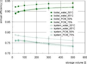The integration of PCM modules (boiler set temp. 65°C in all cases) allows an enhancement of the storage capacity, resulting in a further decrease of the number of start-stop cycles especially with small storage volumes. There are only minor differences between the PCM volume fractions of 50 and 75 %. The integration of PCM modules hardly influences the annual efficiencies of the boiler and the system (Fig. 4, right).

Fig, 4. Gas boiler: annual number of start-stop cycles (left) and annual efficiencies (right) for different
storage volumes for systems with water storage (G2a) and for systems with water storage with integrated

PCM modules (G2b)

Figure 5 shows the number of start-stop cycles and the annual efficiencies for the system G3a (water storage) and the system G3b (bulk PCM storage). Due to the higher storage capacity of the PCM storage (assuming the same volume of 45 litres) in system G3b the number of cycles can be reduced by 50 % compared to system G3a. The annual efficiency of the boiler is also slightly higher, which is a result of the lower amount of heat produced in start-stop operation due to the higher storage capacity.

2. Conclusion

Phase change materials as heat storage theoretically offer an advantage compared to water stores, when the cycling temperature is close around the phase change temperature and the phase change can be used quite often. The other possible application is the use of the subcooling effect for seasonal storage. However, the investigations reported here showed only little advantages for macro-encapsulated PCM modules in combistores, PCM-stores with immersed heat exchangers and for PCM slurries for heat stores in solar combisystems and residential heating systems. The seasonal storage with subcooled PCM could be in principle a good solution. However the technical expenditure for this system is large.

References

[1] A. Abhat, (1983), Low temperature latent heat thermal energy storage: heat storage materials, Solar Energy 30 (1983) 313-332.

[2] W. Streicher, (ed). (2008), Laboratory Prototypes of PCM Storage Units, Report C4, of IEA Solar Heating and Cooling programme — Task 32, “Advanced storage concepts for solar and low energy buildings”, IEA-SHC (http://www. iea-shc. org/task32/publications/index. html)

[3] H. Heimrath, M. Haller, (2008), The Reference Heating System, the Template Solar System, Report A2, of IEA Solar Heating and Cooling programme — Task 32, “Advanced storage concepts for solar and low energy buildings”, IEA-SHC (http://www. iea-shc. org/task32/publications/index. html)

[4] S. Citherlet, J. Bony, (2008), System Simulation Report, System : HEIG-VD-W and HEIG-VD-PCM, Report C6.1, of IEA Solar Heating and Cooling programme — Task 32, “Advanced storage concepts for solar and low energy buildings”, IEA-SHC (http://www. iea-shc. org/task32/publications/index. html)

[5] J. M. Schultz, (2008), System Simulation Report, PCM with supercooling, Report C6.2, of IEA Solar Heating and Cooling programme — Task 32, “Advanced storage concepts for solar and low energy buildings”, IEA-SHC (http://www. iea-shc. org/task32/publications/index. html)

[6] A. Heinz, (2008), System Simulation Report, System: PCM storage to reduce cycling rates for boilers, Report C6.3, of IEA Solar Heating and Cooling programme — Task 32, “Advanced storage concepts for solar and low energy buildings”, IEA-SHC (http://www. iea-shc. org/task32/publications/index. html

T. Koller[18] [19], M. Zetzsche1, Prof. Dr. Dr. H. Mtiller-Steinhagen1,2

1 University of Stuttgart, Institute for Thermodynamics and Thermal Engineering (ITW)

2 Institute of Technical Thermodynamic (ITT), DLR
http://www. itw. uni-stuttgart. de/~www/ITWHomepage/Forschung/Kaelte. html

Abstract

A small ice store has been designed, constructed and experimentally investigated at the

Institute of Thermodynamics and Thermal Engineering (ITW) of the University of Stuttgart [1]. A simulation program based on EES and Matlab was developed which predicts the experimental data well.

Measurements have shown a higher volumetric capacity (56 kWh/m[20]) than expected from published reports (40 — 44 kWh/m3) [2].The present design offers an efficient solution for cold storage at low cost, and low maintenance and operation efforts.

The chosen type of storage is an ice-on-coil system with external melting. While internal melting would result in higher discharging rates, it is nevertheless not a viable option because of particular requirements on operational mode and design of the present heat exchanger.

The ice store was implemented into the cooling system of the institute building and shows good in-service behaviour. Next steps are further development of the storage design, automation of the operational mode and detailed measurements and evaluation of in-service behaviour.

Keywords: Ice Store, Solar Cooling, Ammonia/Water Chiller, Air-Conditioning

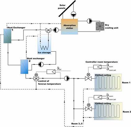
system consisting of absorption chiller, ice storage and solar collector field. This system, which is illustrated in Figure 1, has been taken into operation in spring 2008.

The latest extension of the solar production plant in Marstal means that they in 2008 have a solar fraction of 30% coming from 18.300 m2 of solar collectors combined with a 10.000 m[31] pit heat storage and a 2.000 m3 steel tank. The rest of the fuel is biooil where the production price/MWh is app. 65 €. Marstal has therefore investigated the possibilities of a larger solar fraction. Design cal­culations shows that an extension with another 4.000 m2 solar collectors, a 10.000 m3 steel tank or pit heat storage, a 1,5 MW heat pump (to cool the storages and use outdoor air) will rise the heat production with 4.800 MWh/year and increase the solar/heatpump fraction to 45%. The production price for the extended production is calculated to 66 €/MWh with an annuity factor of 0,1 and without electricity tax. The extension is planned to be realised in 2009.

Investment costs are 2,8 mio. €.

3.1. Strandby

Strandby Varmevsrk is a consumer owned district heating company producing 16.000 MWh/year with natural gas fuelled CHP and boiler. In the summer 2008 Strandby Varmevsrk is implement­ing 8.000 m2 solar collectors, 1.500 m3 steel tank and an absorption heat pump. The solar collectors will cover 18% of the annual heat production and the absorption heat pump will cover another 5%. The absorption heat pump is cooling fluegas from CHP, and boiler and utilising low temperature heat form the solar collectors. The production price for heat is calculated to 55 €/MWh (annuity 0,1).

Investment costs are 2,2 mio. €

The research approach has been based on the combination of virtual prototyping techniques (numerical simulation) and the construction and measurement of experimental set-ups and prototypes by means of ISO procedures.

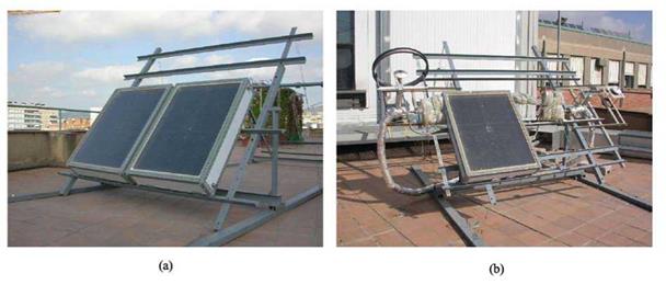
More than 7000 different configurations of ICSs have been evaluated by means of virtual prototyping. Main parameters investigated were: the absorbing surfaces, the covers (from single glazing to transparently insulated covers), different stores (water store, PCM store, hybrid water+PCM store), and different volume of the store. Some of the most interesting configurations in terms of the industrialisation capabilities of the partners, the cost, the thermal performance, and the technical feasibility according to the current state of the technique, have been studied in more detailed resulting into the final OPICS-ICSs developed during the project. Other configurations, however, may also be interesting and may motivate further investigation and development in the frame work of future projects. Some of the configurations studied in the virtual prototyping have been evaluated in more detail, including a detailed design of all the elements, the construction of prototypes, a detailed modelling, and the testing of the prototypes using ISO procedures.

1.1. Solar combisystem modelling

The first step in the study consists in the creation of a reference model of a solar combisystem. The system is designed to provide energy for space heating and domestic hot water for a single-family house. It is installed in a low energy house and does not include any long-term Thermal Energy Storage System (TESS). This reference case has been programmed with the transient system simulation program TRNSYS [2]. This software is a complete and extensible simulation environment for the transient simulation of energy systems, including multi-zone buildings. Its modular structure allows the user to build his own systems, from simple domestic hot water systems to the design of

buildings and their equipments, including control strategies, occupant behaviour, alternative energy systems (wind, solar, photovoltaic, hydrogen systems), etc.

The model of the reference combisystem is divided in several sub-sections as depicted in Fig. 2 :

• the solar collector loop with an area of 20 m2 of evacuated tube collectors and counter flow heat exchanger

• the auxiliary heating loop, comprising an electric heater

• the domestic hot water (DHW) demand module, controlled by a load profile and set to provide 200 L of water at 45°C per day, which is the daily consumption of a five-person family

• the building representation section, which corresponds to a low energy single family house of 191 m2 with a bioclimatic architecture

• the space heating loop, modelled with a radiator

• the weather data processing module, which reads the weather data and calculates direct and diffuse radiation outputs for the surfaces of the building and solar collectors with various orientations and slopes.

Solar collector loop

Evacuated tubes (71)

Weather (109)

Building

Aux pump (803) Aux coldpipe (31)

Space heating

DHW

Fig. 2. Reference solar combisystem layout

This figure is a simplified layout ; all the controllers and regulation devices are omitted.

Fig. 4. Space heating demand of the modelled house

The building has a space heating demand of 37.2 kWh. m-2 in Paris and 15.4 kWh. m-2 in Marseille. If space heating and DHW preparation are both considered, the demand rise to 53.0 kWh. m-2 and 31.1 kWh. m-2 for Paris and Marseille respectively.

Seasonal Storage

Seasonal TES by sorption storage seems to be particularly interesting, because there are no heat losses during the storage period. The stored thermal energy will only be discharged, when the adsorption process will be started. This is only valid, if the sensible heat of the adsorbent is

neglected. About 10 — 15 % of the heat input will be lost by the cooling down of the adsorbent material.

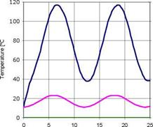
However seasonal storage by sorption systems is strongly influenced by the changes in the ambient temperature between summer and winter. A substantial decrease in the thermal coefficient of performance COPth will be shown in the following example [1]: The charging of the sorption storage will take place in summer time at an ambient temperature of 30 °C (TAC). Discharging will be in winter at -20 °C (TAD). These circumstances lead to a substantial decrease of the ideal ratio of thermal energy output Qout (discharging) and solar input Qin (charging).

In this example the charging and discharging temperature of the storage is 100 °C. In a number of applications the charging temperature is higher than the discharging temperature, which leads to a further decresas in COPth.

If you have a solar application and a Zeolite storage, where you need a charging temperature of at least 160 °C and you are delivering heat to a low temperature heating system running at 40 °C, your thermodynamical maximum COPth can only be 54%.