The experiments are carried out in a box with a square base of 100×100 mm and a height of 150mm. The base of the test cell is made of copper with 5 mm thickness and the lateral sidewalls are made in 4 mm transparent acrylic. The sidewalls are isolated by 30 mm polystyrene coated with 5 mm ceramic fiber. This isolation is removed temporarily each time flow visualization with PIV and Shadowgraph techniques occurs. A precision heater is used to provide uniform heating over the base of the copper test cell at a prescribed temperature. The desired linear salinity gradients are created using the two tanks method described by Oster [9] and Hill [10].

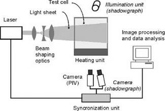
By applying the PIV system the measurement of velocities in the convective regions and the observation of the flow patterns are accomplished. Figure 1 shows the PIV setup. A 10Hz Nd:YAG Q-switched laser with frequency doubled 532 nm wavelength emits a circular light beam, and an optical setup (beam shaping optics) creates a sheet of light with 1 mm thickness and low divergence height. This sheet of light crosses the inspected volume and the light scattered by the seeding particles is visualized by a CCD camera, perpendicular to the light sheet. The seeding particles, hollow glass spheres with an average diameter of 12 pm, are mixed in the aqueous salt (NaCl) solutions before the formation of the stratified layer. The synchronization between the laser and the camera is made by an electronic circuit developed for that purpose. For each PIV acquisition 30 images of particles, exposed to individual frame and with an acquisition rate of 10Hz, are captured. Afterwards, these images are processed using specific software (Dynamic. Studio from Dantec Dynamics A/S). The processing consists in the cross-correlation of each pair of images of particles captured, producing a vector map of the instantaneous velocity field of the field of view. At present study, the field of view of the PIV system is a rectangle with 64 mm height and 84 mm width.

Figure 1 also includes the schematic of the Shadowgraph setup. This method makes use of a 100W halogen lamp that projects the emitted light on a semi-transparent screen placed near the test cell. This allows a near to 1:1 relation between the object and the projected shadowgraph image. Using this technique the positions of the interface zones can be identified, and their evolution analyzed. The shadowgraphs images that capture the sudden changes on the medium refractive index are visualized by a CCD camera, alternating with the PIV analysis. Both the CCD cameras have 640×480 pixels and 8.6×8.3 pm pixel pitch.

The vertical temperature and concentration of salt distributions near the centre of the test cell are measured during the experiments with a Micro Scale Conductivity and Temperature Instrument, MSCTI (from Precision Measurement Engineering, Inc) [11]. From time to time, this probe, with high special resolution (1 mm) and fast response, is made to move slowly through the system, using a computer controlled linear translation axis to command the step movement of the MSCTI and the translation velocity. The measurements were performed with a 1 mm step and with a velocity translation of 0.1 mm/s, or 0.05 mm/s. Empirical equations are used to convert conductivity data, at a giving temperature measured simultaneously, to salt concentration [12]. A vertical temperature probe rake, consisting of 16 calibrates Pt100 probes mounted at approximately 5 mm intervals, allowed the continuous measurement of the evolution of the vertical temperature profile during the experiments.